The proposed simplification algorithm (Density Preserving Hierarchical EM, DPHEM) is applied on synthetic data and real applications. Comparison is implemented with other 3 most related algorithms: HEM, VKL and L2U.
On Synthetic 2d GMMs
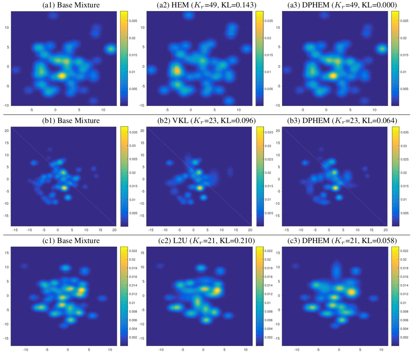
Examples of reduced mixture models using different approaches. Each row compares DPHEM with a baseline method and shows a typical difference. The base mixture model contains 2500 components, and the reduced mixture contains Kr components. KL is the KL divergence between the base mixture and the reduced mixture.
On Mixture KDE Reduction
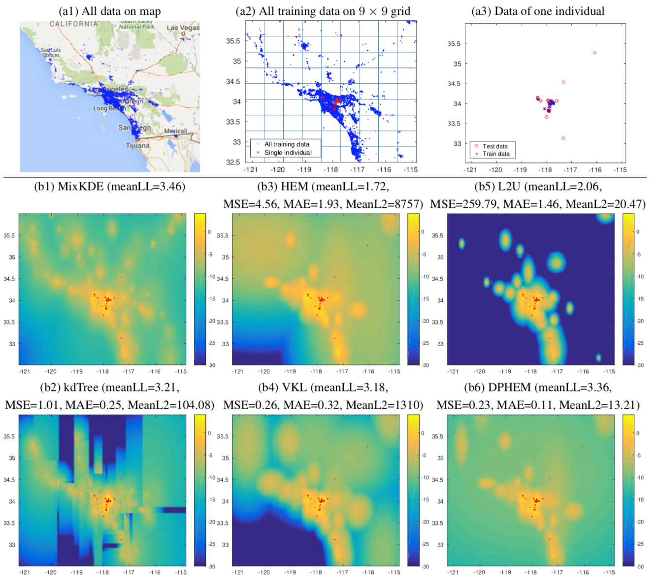
Example of human location modeling: (a1) All check-in records used for training and testing on map; (a2) All training and testing of one selected individual on a 9 × 9 grid; (a3) The individual’s training and testing data. (b) Log-likelihood map of the individual’s spatial distribution estimated from check-in records with mixture KDE model (MixKDE) and the simplified models with Kr = 90. Red dots are the test events of this individual. meanLL is the average log-likelihood of the test events. MSE and MAE are the mean squared error and mean absolute error between the test event log-likelihoods predicted by the original MixKDE and the approximate model, while MeanL2 is the mean L2 distance between test event likelihoods. For better visualiza- tion, log-likelihood values are truncated at -30.
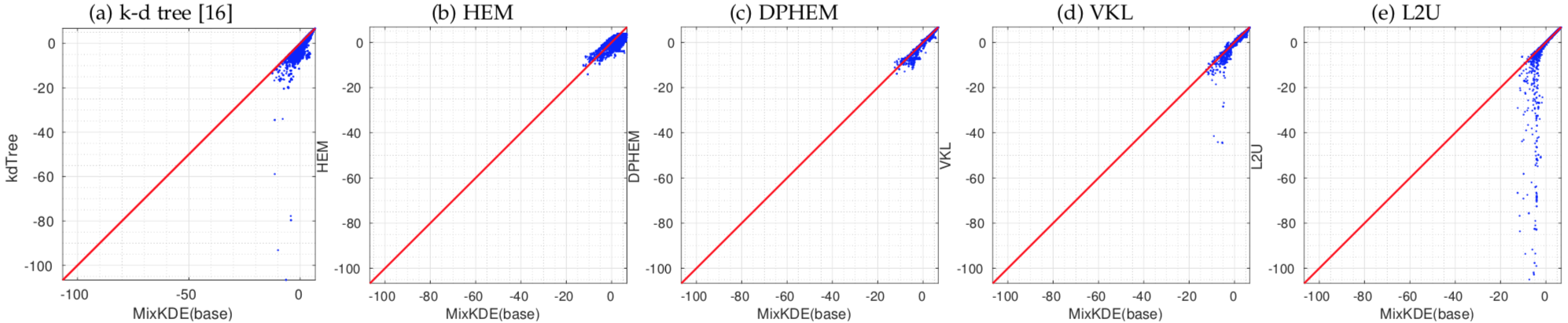
Pair-wise comparison of the log-likelihood of test events on mixture KDE and reduced mixture models with Kr=90 using different approaches.
On Visual Tracking
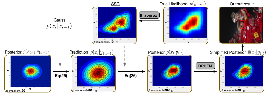
A typical first-order Markov model is applied to form our tracking framework with GMM posteriors. In order to work under an unified recursive Bayesian filtering framework, the appearance model returned as scores at discrete locations is also approximated as a sum of scaled Gaussian (SSG). DPHEM is applied whenever the number of mixture components exceeds a predefined value. Maximum a Posterior is used to determine the state of target at each step.
Pipeline for visual tracking using GMM posteriors and density simplification.
(add an example tracking video)
On Vehicle Self-localization
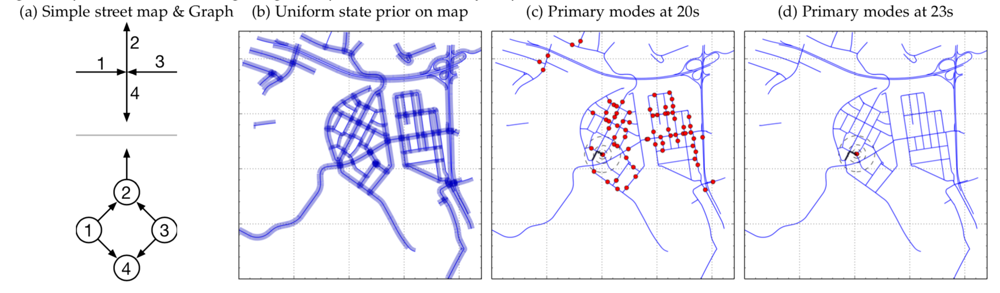
In [Brubaker et al., 2016], they proposed a probabilistic model for vehicle self-localization using roof-mounted cameras and a map of the driving environment. The map is represented as a graph, and probabilistic models describe how the vehicle can traverse the graph. Recursive Bayesian filtering is used to infer the posterior probability of the vehicle’s states (location and orientation) on the map, given the visual odometry (observed displacement and orientation change) calculated from the cameras.
An example of street map and graph representation, and the inference results for the vehicle’s state on the map. The vehicle is considered as localized when there is a single primary mode for 10 contiguous frames.
Applying simplification to the posterior can save more than half the computing time, and DPHEM is faster than the other simplification methods.
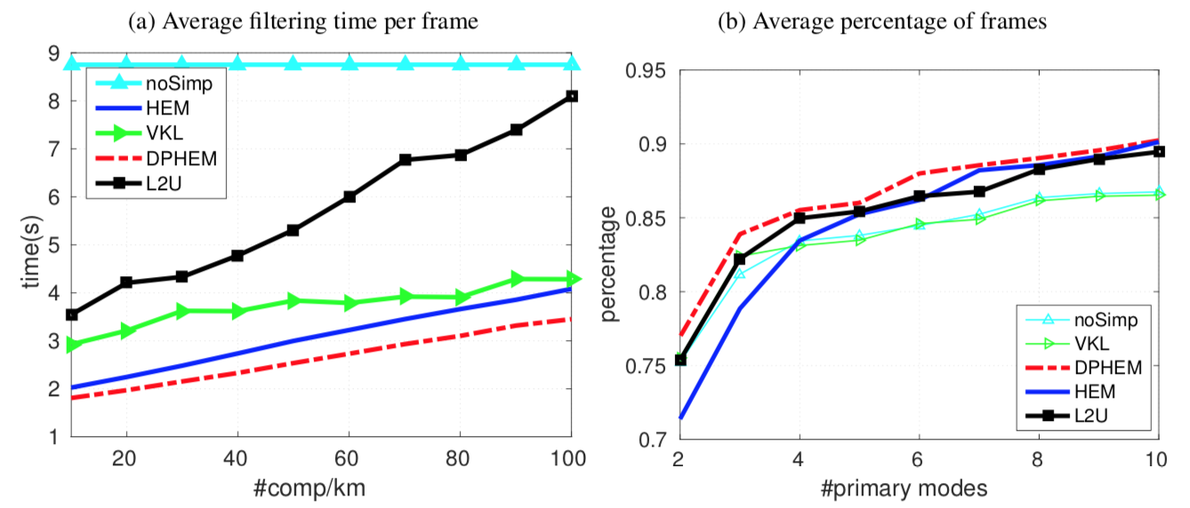
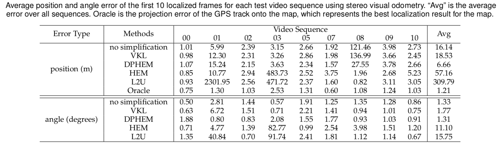
DPHEM has higher percentage of frames having less primary modes, which means the ambiguity decreases faster than other methods, and good suggestions about the vehicle’s location can be proposed at earlier times. Even though the number of primary modes decreases faster, the localization error shown in Table shows that the accuracy does not diminish.
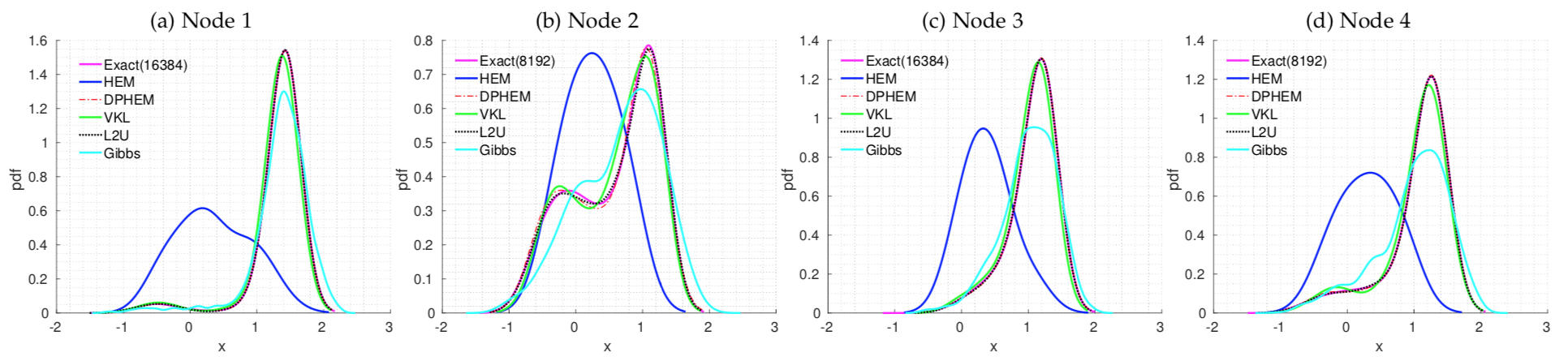
On Synthetic Belief Propagation
In order to compare the simplified belief with those from exact inference, we generate an undirected 4-node graph, with self-potential being 2-component GMM and edge-potential being a single Gaussian. Here shows the marginal density (belief) at each node after the 3rd iteration of belief propagation. The number of components in the exact marginal density at each node is shown in the legend. Gibbs sampling uses 1024 samples, while simplification methods use Kr = 4.